Mamba 🐍

The Mamba model represents a significant advancement in the field of sequence modeling, particularly in addressing the computational inefficiencies associated with Transformer architectures, developed by Albert Gu and Tri Dao, mamba is a structured state space model (SSM) designed to offer linear scaling with sequence length while retaining or even surpassing the performance of traditional Transformers on various tasks, including language, audio, and genomics.

Motivation

Modern foundational models in deep learning are predominantly built on Transformer architectures, which excel due to their self-attention mechanism, this allows them to route information densely within a context window, modeling complex data effectively, however the quadratic scaling of self-attention with sequence length poses significant computational challenges, particularly for long sequences, various alternatives, such as linear attention, gated convolution, and other SSMs, have been proposed to mitigate these inefficiencies but have struggled to match the performance of Transformers, especially in content-based reasoning and discrete modalities like text.

Core Innovations

Selective State Space Models

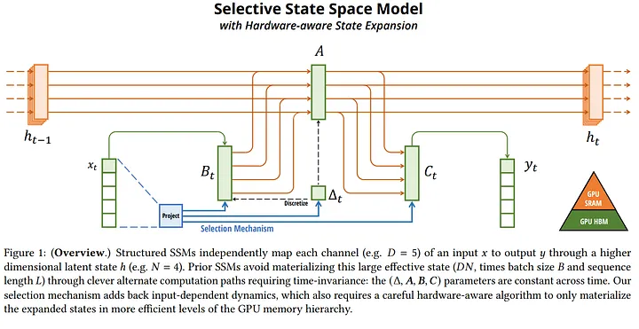
Mamba introduces selective state space models, an innovative enhancement to the traditional SSM framework, the key innovation here is parameterizing SSM parameters based on the input, enabling the model to dynamically decide which information to propagate or forget at each timestep, this selective mechanism allows Mamba to maintain relevant information over long sequences, addressing the inherent weakness of prior SSMs in handling discrete and information-dense data.

Hardware-Aware Parallel Algorithm

A significant challenge with the input-dependent parameterization of SSMs is the computational inefficiency it introduces, as it prevents the use of efficient convolutions , mamba overcomes this by employing a hardware-aware parallel algorithm that computes the model in a recurrent mode without materializing the expanded state, this approach leverages the GPU memory hierarchy to perform efficient computations, achieving faster execution than previous methods and maintaining linear scaling with sequence length.

Architectural Design

Mamba’s architecture is streamlined by integrating selective state spaces into a simplified neural network design, eliminating the need for attention or multi-layer perceptron (MLP) blocks typically found in Transformers. this homogeneous design results in a model that not only simplifies the architecture but also improves computational efficiency and throughput.

State Space Models

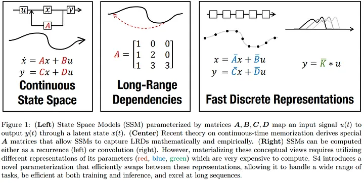
Mamba builds upon the foundation of structured state space sequence models (S4), which combine elements of recurrent neural networks (RNNs) and convolutional neural networks (CNNs) .

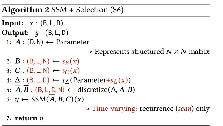
These models are defined by four parameters: Δ, A, B, and C, which dictate the sequence-to-sequence transformation through a latent state, the transformation involves two stages: discretization of continuous parameters and computation as either a linear recurrence or a global convolution.

Linear Time Invariance (LTI)

Traditional SSMs are linear time-invariant (LTI), meaning their parameters remain constant across time steps, this property facilitates efficient computation as convolutions but limits the model’s ability to adapt dynamically to different inputs, mamba addresses this limitation by introducing input-dependent dynamics, enhancing the model’s flexibility and performance on complex tasks.

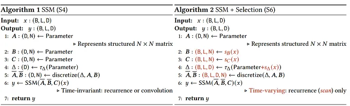
Structured and Selective Computation

To handle the increased complexity introduced by selective state spaces, Mamba employs a structured approach to the A matrix, often using a diagonal structure to simplify computations, this structured approach ensures that the model scales efficiently with input size and sequence length, maintaining computational feasibility even for large-scale tasks.

Mamba block

The Mamba architecture is a simplified SSM architecture that combines the H3 block (which is the basis of most SSM architectures) with the ubiquitous MLP block of modern neural networks, instead of interleaving these two blocks, Mamba repeats the block homogenously.

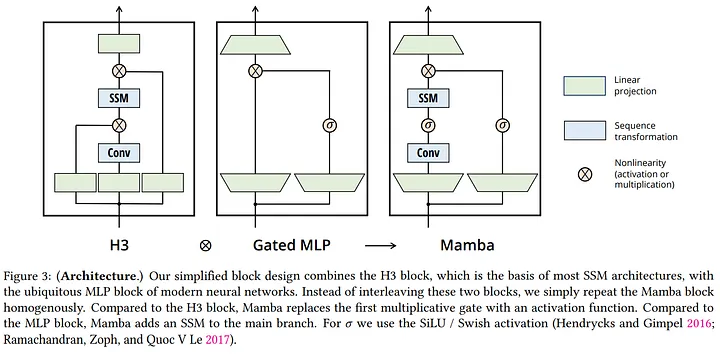
1 . Input Projection: the input is projected to a higher dimension (D*E), where E is the expansion factor (usually 2).

2 . Sequence Transformation:

• Mamba-S6 (Selective SSM): the main branch performs a selective structured state space transformation (S6) , this involves input-dependent parameters (Δ, B, C) and a hardware-aware recurrent scan algorithm.

• Local Convolution: an optional local convolution is applied before the S6 layer (similar to H3).

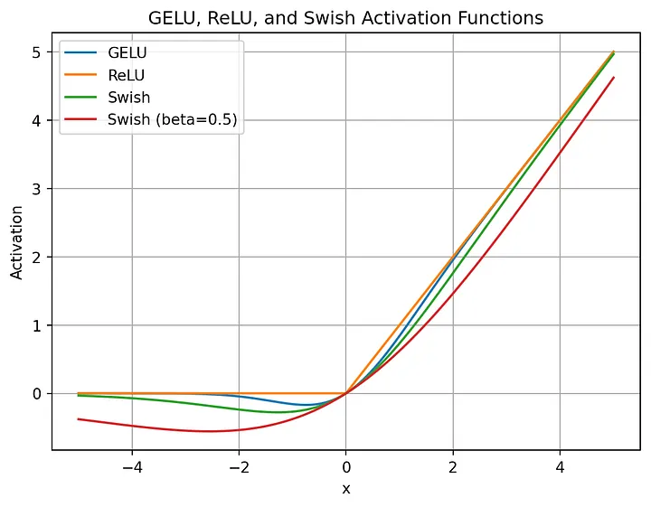
3 . Nonlinearity (SiLU/Swish): A SiLU/Swish activation function is applied to the output of the sequence transformation.

4 . Output Projection: the output is projected back to the original dimension (D).

5 . Gated MLP: a standard MLP with an expansion factor of E (usually 2) and SiLU/Swish activation function is used as a second branch, this is similar to the “SwiGLU” variant.

6 . Addition: the outputs from the main branch and the MLP branch are added together.

7 . Normalization: An optional normalization layer (LayerNorm) is applied to the final output.

---

Mamba represents a paradigm shift in sequence modeling, addressing the limitations of traditional Transformers through innovative core components and architectural design, at its heart Mamba utilizes Selective State Space Models (S-SSMs) which dynamically adjust parameters based on the input to retain or forget information selectively, this flexibility allows Mamba to handle discrete data modalities and long-range dependencies more effectively than its predecessors , also the Hardware-Aware Parallel Algorithm ensures that these complex computations remain efficient, leveraging the GPU memory hierarchy for optimal performance .

Mamba’s architectural simplicity, combining state space models with linear time invariance and structured computation, forms a robust foundation for scalable and high-throughput sequence modeling , the modular Mamba block seamlessly integrates these components, providing a versatile framework that excels across various tasks, from language processing to genomics.

as we delve into the code, we will build Mamba block by block from scratch and train it on our Algerian Darija , this hands-on approach will demonstrate how Mamba’s unique architecture can be adapted to make the model proficient in understanding and generating Algerian Darija, showcasing its versatility and efficiency in real-world applications.

---

Code Time

Imports essential dependencies

Here in this block we imports essential libraries and modules for building our mamba model in pytorch.

from __future__ import annotations
import math
import json
import torch
import torch.nn as nn
import torch.nn.functional as F
from dataclasses import dataclass
from einops import rearrange, repeat, einsum
from typing import Union
from torch.utils.data import Dataset, DataLoader
from transformers import get_scheduler

Load , train and prepare our Tokenizer

In this code block we’re preparing a new tokenizer tailored for training a model on Darija, starting with a base tokenizer and then customizing it with additional tokens and configurations.

In the first step, we define the get_training_corpus function to load our training data from a text file, this function uses load_dataset from the datasets library to read the data and yields chunks of 1000 text samples at a time , after that we initialize the base_tokenizer from a pre-trained model (state-spaces/mamba-130m-hf) using the AutoTokenizer class from Hugging Face.

from transformers import AutoTokenizer
from datasets import load_dataset

# Function to get training data
def get_training_corpus():
    dataset = load_dataset("text", data_files={"train": "cleaned_data.txt"})
    for i in range(0, len(dataset["train"]), 1000):
        yield dataset["train"][i : i + 1000]["text"]

# Initialize the base tokenizer
base_tokenizer = AutoTokenizer.from_pretrained("state-spaces/mamba-130m-hf")

# Train the new tokenizer
new_tokenizer = base_tokenizer.train_new_from_iterator(get_training_corpus(), 
                   vocab_size=1000) # you change it to match your need

# Save the new tokenizer
new_tokenizer.save_pretrained("new_tokenizer")

new_tokenizer.pad_token = new_tokenizer.eos_token

fim_prefix_token = "<fim_prefix>"
fim_middle_token = "<fim_middle_token>"
fim_suffix_token = "<fim_suffix_token>"
fim_pad_token = "<fim_pad>"

# Get the FIM-specific tokens and get their token ids
new_tokenizer.add_tokens(
    [
        fim_prefix_token,
        fim_middle_token,
        fim_middle_token,
        fim_pad_token,
    ]
)
prefix_tok_id = new_tokenizer.convert_tokens_to_ids(fim_prefix_token)
middle_tok_id = new_tokenizer.convert_tokens_to_ids(fim_middle_token)
suffix_tok_id = new_tokenizer.convert_tokens_to_ids(fim_middle_token)
pad_tok_id = None

fim_tokens = [prefix_tok_id, middle_tok_id, suffix_tok_id]


# If truncate_or_pad is on, also get pad token id
truncate_or_pad = True
if truncate_or_pad:
    pad_tok_id = new_tokenizer.convert_tokens_to_ids(fim_pad_token)
    fim_tokens.append(pad_tok_id)

Next, we create a new tokenizer instance with a specific vocabulary size of 1000 by calling train_new_from_iterator on the base_tokenizer with the get_training_corpus function as input, this step fine-tunes the base tokenizer to better represent the specific vocabulary of the Darija data. Following this, we save the new tokenizer to a directory named new_tokenizer, allowing us to reuse it for future tasks.

After saving the tokenizer we modify its configuration by setting the pad_token to the same as the eos_token to ensure consistent padding behavior , next we define several FIM tokens and add them to the tokenizer’s vocabulary, these FIM tokens are crucial for special instructions and are appended to the tokenizer’s vocabulary.

Finally we determine the token IDs for the newly added FIM tokens and manage the padding token ID if truncate_or_pad is set to True ,this includes adding the fim_pad_token to the list of FIM tokens and converting it to its corresponding ID.

Create custom Dataset Loader class

The TextDataset class is defined as a subclass of Dataset from pytorch. this class is designed to manage and pre-process text data for training a model , this custom dataset class is crucial for setting up the data pipeline for training models, ensuring that the text data is appropriately formatted and ready for processing.

# Custom Dataset Class
class TextDataset(Dataset):
    def __init__(self, file_path, tokenizer, context_len=384):
        self.tokenizer = tokenizer
        self.context_len = context_len

        # Load and tokenize data
        with open(file_path, 'r', encoding='utf-8') as f:
            self.data = f.read()

        self.tokens = tokenizer(self.data, return_tensors='pt', truncation=True, padding='max_length', max_length=context_len)

    def __len__(self):
        return len(self.tokens['input_ids'])

    def __getitem__(self, idx):
        return {
            'input_ids': self.tokens['input_ids'][idx],
            'labels': self.tokens['input_ids'][idx] # don't worry brother we will shift it later in the training loop
        }

Define model HyperParameters

ModelArgs class encapsulates the mamba model hyperparameters, making it easier to manage and adjust settings as needed.

@dataclass
class ModelArgs:
    d_model: int
    n_layer: int
    vocab_size: int
    d_state: int = 16
    expand: int = 2
    dt_rank: Union[int, str] = 'auto'
    d_conv: int = 4
    pad_vocab_size_multiple: int = 8
    conv_bias: bool = True
    bias: bool = False

    def __post_init__(self):
        self.d_inner = int(self.expand * self.d_model)

        if self.dt_rank == 'auto':
            self.dt_rank = math.ceil(self.d_model / 16)

        if self.vocab_size % self.pad_vocab_size_multiple != 0:
            self.vocab_size += (self.pad_vocab_size_multiple
                                - self.vocab_size % self.pad_vocab_size_multiple)

RMS Normalization Layer

First we initialize the class which inherits from nn.Module, setting up the normalization parameters, in the init method, we define eps (a small value to prevent division by zero) and weight, which is a learnable parameter initialized to ones with the size of the model dimension d_model.

class RMSNorm(nn.Module):
    def __init__(self,
                 d_model: int,
                 eps: float = 1e-5):
        super().__init__()
        self.eps = eps
        self.weight = nn.Parameter(torch.ones(d_model))


    def forward(self, x):
        output = x * torch.rsqrt(x.pow(2).mean(-1, keepdim=True) + self.eps) * self.weight

        return output

Then, in the forward method, the actual normalization happens: it takes an input tensor x and computes the Root Mean Square (RMS) normalization, specifically it squares the input values, computes their mean along the last dimension, adds the epsilon value for stability, and then takes the reciprocal square root, this result is multiplied element-wise with the input and the learnable weight parameter, producing the normalized output, this technique stabilizes training and ensures that the output values maintain a consistent scale, which helps in training deep neural networks efficiently.

Create The Residual Block

In the ResidualBlock class, which inherits from nn.Module, we create a building block for neural networks that includes a normalization step and a residual connection, ensuring stability and efficiency during training, in the init method, we initialize the block with a MambaBlock for mixing and an RMSNorm for normalization, using parameters from ModelArgs, in the forward method, the input tensor x undergoes normalization first through RMSNorm, then is processed by the MambaBlock, and finally, the original input x is added back to the processed output, forming a residual connection.

class ResidualBlock(nn.Module):
    def __init__(self, args: ModelArgs):
        """Simple block wrapping Mamba block with normalization and residual connection."""
        super().__init__()
        self.args = args
        self.mixer = MambaBlock(args)
        self.norm = RMSNorm(args.d_model)


    def forward(self, x):
        output = self.mixer(self.norm(x)) + x

        return output

This approach helps in preserving the original input information and stabilizes gradient flow during backpropagation, making the network more robust and easier to train, the implementation here is designed to be simple and numerically equivalent to the official implementation, which chains residual blocks differently for performance reasons.

Create the Mamba Block ( ssm / selective scan )

in the MambaBlock class which is part of a our mamba architecture, we define a complex module based on the Mamba paper.

initially the init method sets up the necessary layers, including a linear layer for input projection, a 1D convolutional layer, and several other linear layers for specific transformations , additionally parameters A and D are initialized, which will be used in the state-space model.

class MambaBlock(nn.Module):
    def __init__(self, args: ModelArgs):
        super().__init__()
        self.args = args

        self.in_proj = nn.Linear(args.d_model, args.d_inner * 2, bias=args.bias)

        self.conv1d = nn.Conv1d(
            in_channels=args.d_inner,
            out_channels=args.d_inner,
            bias=args.conv_bias,
            kernel_size=args.d_conv,
            groups=args.d_inner,
            padding=args.d_conv - 1,
        )

        # x_proj takes in `x` and outputs the input-specific Δ, B, C
        self.x_proj = nn.Linear(args.d_inner, args.dt_rank + args.d_state * 2, bias=False)

        # dt_proj projects Δ from dt_rank to d_in
        self.dt_proj = nn.Linear(args.dt_rank, args.d_inner, bias=True)

        A = repeat(torch.arange(1, args.d_state + 1), 'n -> d n', d=args.d_inner)
        self.A_log = nn.Parameter(torch.log(A))
        self.D = nn.Parameter(torch.ones(args.d_inner))
        self.out_proj = nn.Linear(args.d_inner, args.d_model, bias=args.bias)


    def forward(self, x):

        (b, l, d) = x.shape

        x_and_res = self.in_proj(x)  # shape (b, l, 2 * d_in)
        (x, res) = x_and_res.split(split_size=[self.args.d_inner, self.args.d_inner], dim=-1)

        x = rearrange(x, 'b l d_in -> b d_in l')
        x = self.conv1d(x)[:, :, :l]
        x = rearrange(x, 'b d_in l -> b l d_in')

        x = F.silu(x)

        y = self.ssm(x)

        y = y * F.silu(res)

        output = self.out_proj(y)

        return output


    def ssm(self, x):

        (d_in, n) = self.A_log.shape

        # Compute ∆ A B C D, the state space parameters.
        #     A, D are input independent (see Mamba paper [1] Section 3.5.2 "Interpretation of A" for why A isn't selective)
        #     ∆, B, C are input-dependent (this is a key difference between Mamba and the linear time invariant S4,
        #                                  and is why Mamba is called **selective** state spaces)

        A = -torch.exp(self.A_log.float())  # shape (d_in, n)
        D = self.D.float()

        x_dbl = self.x_proj(x)  # (b, l, dt_rank + 2*n)

        (delta, B, C) = x_dbl.split(split_size=[self.args.dt_rank, n, n], dim=-1)  # delta: (b, l, dt_rank). B, C: (b, l, n)
        delta = F.softplus(self.dt_proj(delta))  # (b, l, d_in)

        y = self.selective_scan(x, delta, A, B, C, D)  # This is similar to run_SSM(A, B, C, u) in The Annotated S4 [2]

        return y


    def selective_scan(self, u, delta, A, B, C, D):

        (b, l, d_in) = u.shape
        n = A.shape[1]

        # Discretize continuous parameters (A, B)
        # - A is discretized using zero-order hold (ZOH) discretization (see Section 2 Equation 4 in the Mamba paper [1])
        # - B is discretized using a simplified Euler discretization instead of ZOH. From a discussion with authors:
        #   "A is the more important term and the performance doesn't change much with the simplification on B"
        deltaA = torch.exp(einsum(delta, A, 'b l d_in, d_in n -> b l d_in n'))
        deltaB_u = einsum(delta, B, u, 'b l d_in, b l n, b l d_in -> b l d_in n')

        # Perform selective scan (see scan_SSM() in The Annotated S4 [2])
        # Note that the below is sequential, while the official implementation does a much faster parallel scan that
        # is additionally hardware-aware (like FlashAttention).
        x = torch.zeros((b, d_in, n), device=deltaA.device)
        ys = []
        for i in range(l):
            x = deltaA[:, i] * x + deltaB_u[:, i]
            y = einsum(x, C[:, i, :], 'b d_in n, b n -> b d_in')
            ys.append(y)
        y = torch.stack(ys, dim=1)  # shape (b, l, d_in)

        y = y + u * D

        return y

in the forward method input x undergoes initial projection and splitting into two parts, followed by a convolutional operation and activation function, the key part ssm computes the state-space parameters and runs the selective scan algorithm on the input, combining state-space dynamics with input-specific parameters , this algorithm is implemented in selective_scan, where continuous parameters are discretized and a sequence of operations updates the state and computes the output sequentially, the final result is projected back to the original input shape and returned as the output of the block.

Let’s combine all pieces together

in Mamba class we implement the full architecture for the Mamba model, following the design principles from the Mamba paper.

In the first step, the init method initializes the model by setting up an embedding layer for converting token IDs to dense representations and a series of ResidualBlock layers for the core processing, based on the number of layers specified in the args object ( we are building here the mamba-130m ) .

After that, it applies RMSNorm for final normalization of the outputs before projecting them to vocabulary size through the lm_head layer, which also shares weights with the embedding layer to align the input and output representations (a technique known as weight tying).

Next the _init_weights method sets up the weights for different layers to ensure the model starts with suitable initial values, using techniques like Xavier uniform initialization for linear layers and normal distribution for embeddings ( in case we want to train it from scratch ).

During the forward pass, the model starts by embedding the input token IDs into dense vectors.

Following this, it processes these vectors through a series of residual blocks that perform transformations and introduce non-linearity.

After the residual blocks, the model applies RMSNorm for final layer normalization before the final linear layer (lm_head) generates the logits over the vocabulary for each token position.

class Mamba(nn.Module):
    def __init__(self, args: ModelArgs):
        """Full Mamba model."""
        super().__init__()
        self.args = args

        self.embedding = nn.Embedding(args.vocab_size, args.d_model)
        self.layers = nn.ModuleList([ResidualBlock(args) for _ in range(args.n_layer)])
        self.norm_f = RMSNorm(args.d_model)

        self.lm_head = nn.Linear(args.d_model, args.vocab_size, bias=False)
        self.lm_head.weight = self.embedding.weight  # Tie output projection to embedding weights.
                                                     # See "Weight Tying" paper
        self.apply(self._init_weights)

    def _init_weights(self, module):
        if isinstance(module, nn.Linear):
            nn.init.xavier_uniform_(module.weight)
            if module.bias is not None:
                nn.init.zeros_(module.bias)
        elif isinstance(module, nn.Embedding):
            nn.init.normal_(module.weight, mean=0.0, std=0.02)
        elif isinstance(module, RMSNorm):
            nn.init.ones_(module.weight)
        elif isinstance(module, nn.MultiheadAttention):
            nn.init.xavier_uniform_(module.in_proj_weight)
            if module.in_proj_bias is not None:
                nn.init.zeros_(module.in_proj_bias)
            nn.init.xavier_uniform_(module.out_proj.weight)
            if module.out_proj.bias is not None:
                nn.init.zeros_(module.out_proj.bias)


    def forward(self, input_ids):

        x = self.embedding(input_ids)

        for layer in self.layers:
            x = layer(x)

        x = self.norm_f(x)
        logits = self.lm_head(x)

        return logits


    @staticmethod
    def from_pretrained(pretrained_model_name: str):
        """Load pretrained weights from HuggingFace into model.

                * 'state-spaces/mamba-2.8b-slimpj'
                * 'state-spaces/mamba-2.8b'
                * 'state-spaces/mamba-1.4b'
                * 'state-spaces/mamba-790m'
                * 'state-spaces/mamba-370m'
                * 'state-spaces/mamba-130m'

        """
        from transformers.utils import WEIGHTS_NAME, CONFIG_NAME
        from transformers.utils.hub import cached_file

        def load_config_hf(model_name):
            resolved_archive_file = cached_file(model_name, CONFIG_NAME,
                                                _raise_exceptions_for_missing_entries=False)
            return json.load(open(resolved_archive_file))


        def load_state_dict_hf(model_name, device=None, dtype=None):
            resolved_archive_file = cached_file(model_name, WEIGHTS_NAME,
                                                _raise_exceptions_for_missing_entries=False)
            return torch.load(resolved_archive_file, weights_only=True, map_location='cpu', mmap=True)

        config_data = load_config_hf(pretrained_model_name)
        args = ModelArgs(
            d_model=config_data['d_model'],
            n_layer=config_data['n_layer'],
            vocab_size=config_data['vocab_size']
        )
        model = Mamba(args)

        state_dict = load_state_dict_hf(pretrained_model_name)
        new_state_dict = {}
        for key in state_dict:
            new_key = key.replace('backbone.', '')
            new_state_dict[new_key] = state_dict[key]
        model.load_state_dict(new_state_dict)

        return model

The from_pretrained static method provides a way to load pre-trained weights for the Mamba model from the Hugging Face Model Hub, it retrieves the model configuration and state dictionary from the Hub, then it initializes a new Mamba instance with these configurations and loads the weights, adjusting the state dictionary to fit the model’s expected format , this setup allows users to quickly obtain a pre-trained Mamba model for their tasks ( in case we want to do fine-tuning or continual pre-training -starting the training from existing checkpoint- ).

Lets Load our Mamba model

here’s a clear and concise explanation of how to initialize the Mamba model with weights from scratch using the ModelArgs class, this is the first way to create a Mamba model, focusing on setting up the model with specific hyperparameters.

"""
mamba-370m : 

        d_model: 1024
        n_layer: 48
        vocab_size: 50280
        d_state: 4096
        expand: 4
        d_conv: 4

mamba-130m : 

        d_model: 768
        n_layer: 24
        vocab_size: 50280
        d_state: 3072
        expand: 4
        d_conv: 4

There is more model sizes like (1.4b and 2.8b)
"""

args = ModelArgs(
    d_model=768,            # Hidden dimension size
    n_layer=24,             # Number of layers
    vocab_size=50280,       # Vocabulary size
    d_state=3072,           # Latent state dimension
    expand=4,             # Expansion factor
    dt_rank='auto',       # Rank of delta
    d_conv=4,             # Convolution kernel size
    pad_vocab_size_multiple=8,
    conv_bias=True,
    bias=False
)
model = Mamba(args)

This approach allows for a customized setup for different training needs.

We start by specifying the pre-trained model checkpoint name, and then we use the from_pretrained method to create a Mamba model initialized with weights from that checkpoint, this approach leverages existing pre-trained knowledge, allowing us to fine-tune the model or use it for specific tasks without starting from scratch.

"""
* state-spaces/mamba-2.8b-slimpj
* state-spaces/mamba-2.8b
* state-spaces/mamba-1.4b
* state-spaces/mamba-790m
* state-spaces/mamba-370m
* state-spaces/mamba-130m
"""

pretrained_model_name = 'state-spaces/mamba-130m'
model = Mamba.from_pretrained(pretrained_model_name)

The Args class sets up the training environment for the model, it specifies paths for the dataset and evaluation data, a learning rate of 1e-4, 100 epochs, a context length of 384 for token sequences, and batch sizes for training and validation, it also selects a GPU if available; otherwise it defaults to the CPU.

class Args:
    # you can change it to match your setup 
    dataset_path = "cleaned_data.txt" 
    eval_path = "validation.txt"
    lr = 1e-4
    epochs = 100
    context_len = 384 
    train_batch_size = 8 
    valid_batch_size = 8
    device = torch.device("cuda:0" if torch.cuda.is_available() else "cpu")

The TextDataset class creates train_dataset and eval_dataset using paths from Args and the new_tokenizer, these datasets are then loaded into train_dataloader and eval_dataloader for batching .

# Load dataset
train_dataset = TextDataset(Args.dataset_path, new_tokenizer, context_len=Args.context_len)
train_dataloader = DataLoader(train_dataset, batch_size=Args.train_batch_size, shuffle=False)

eval_dataset = TextDataset(Args.eval_path, new_tokenizer, context_len=Args.context_len)
eval_dataloader = DataLoader(eval_dataset, batch_size=Args.valid_batch_size, shuffle=False)

# Optimizer and Scheduler
optimizer = torch.optim.AdamW(model.parameters(), lr=Args.lr)
scheduler = get_scheduler(
    "cosine", optimizer=optimizer, num_warmup_steps=100, num_training_steps=len(train_dataloader) * Args.epochs
)

Next an AdamW optimizer is set up for model training with a learning rate from Args, and a cosine scheduler adjusts the learning rate over the course of the training based on the number of steps and warm-up period.

Lets start the Training phase

we start by moving the model to the specified device and starts training for the number of epochs defined in Args.

model.to(Args.device)
for epoch in range(Args.epochs):
    model.train()
    total_loss = 0

    for batch in train_dataloader:
        batch = {k: v.to(Args.device) for k, v in batch.items()}

        outputs = model(batch['input_ids'])

        # Compute the loss manually
        shift_logits = outputs[..., :-1, :].contiguous()
        shift_labels = batch['labels'][..., 1:].contiguous()
        loss_fct = torch.nn.CrossEntropyLoss()
        loss = loss_fct(shift_logits.view(-1, shift_logits.size(-1)), shift_labels.view(-1))

        loss.backward()
        optimizer.step()
        scheduler.step()
        optimizer.zero_grad()

        total_loss += loss.item()

    print(f"Epoch {epoch+1}/{Args.epochs}, Loss: {total_loss / len(train_dataloader)}")
    # Evaluation
    model.eval()
    total_eval_loss = 0

    with torch.no_grad():
        for batch in eval_dataloader:
            batch = {k: v.to(Args.device) for k, v in batch.items()}

            outputs = model(batch['input_ids'])

            # Compute the loss manually
            shift_logits = outputs[..., :-1, :].contiguous()
            shift_labels = batch['labels'][..., 1:].contiguous()
            loss_fct = torch.nn.CrossEntropyLoss()
            loss = loss_fct(shift_logits.view(-1, shift_logits.size(-1)), shift_labels.view(-1))

            total_eval_loss += loss.item()

    avg_eval_loss = total_eval_loss / len(eval_dataloader)
    print(f"Epoch {epoch+1}/{Args.epochs}, Evaluation Loss: {avg_eval_loss}")
    model_save_path = "mamba_darija.pt"
    torch.save(model.state_dict(), model_save_path)
    print("Training complete!")

For each epoch it trains the model by computing the loss, performing backpropagation, updating the weights, and adjusting the learning rate. after training it evaluates the model’s performance on the validation data, calculates the average evaluation loss, and saves the trained model’s state.

The Inference time

max_length = 30
num_return_sequences = 10


tokens = new_tokenizer.encode("راك ")
tokens = torch.tensor(tokens , dtype=torch.long)
tokens = tokens.unsqueeze(0).repeat(num_return_sequences, 1)

x = tokens.to(Args.device)

while x.size(1) < max_length:

    with torch.no_grad():
        outputs = model(x)
        logits = outputs[0] if isinstance(outputs, tuple) else outputs
        logits = logits[:, -1, :]
        probs = F.softmax(logits, dim=-1)
        topk_probs, topk_indices = torch.topk(probs, 50, dim=-1)

        ix = torch.multinomial(topk_probs, 1)
        xcol = torch.gather(topk_indices, -1, ix)
        x = torch.cat((x, xcol), dim=1)

# print the generated text
for i in range(num_return_sequences):
    tokens = x[i, :max_length].tolist()
    decoded = new_tokenizer.decode(tokens, skip_special_tokens=True)
    print(">", decoded)

This code generates text sequences based on a given prompt , it starts by encoding the prompt and creating multiple copies of it, in a loop it predicts the next token appends it to the sequence, and repeats until the desired length is reached , after generating the sequences, it decodes and prints them.

---