Building a Mamba-Transformer from Scratch

Combining Mamba architecture with Transformer architecture represents an innovative approach in deep learning that leverages the strengths of both architectures to address their respective limitations. The Mamba architecture, known for its efficiency in sequential data processing and inherent ability to encode positional information, complements the powerful self-attention mechanism of Transformers, which excels in capturing long-range dependencies but can be computationally intensive. By integrating these architectures, hybrid models like Jamba, MambaVision, and Mambaformer achieve enhanced performance, efficiency, and scalability across various domains such as language modeling, computer vision, and time series forecasting. This synergy not only improves computational and memory efficiency but also results in state-of-the-art performance in complex tasks, demonstrating the significant advantages of combining these two cutting-edge architectures
Mamba Architecture
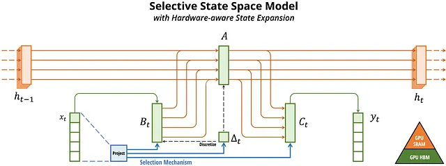
Mamba is an innovative sequence modeling architecture designed to address some of the limitations found in traditional Transformers, unlike Transformers which use self-attention mechanisms to capture dependencies across long sequences but are computationally intensive, Mamba utilizes selective state space models (SSMs) , these models are particularly efficient for processing sequential data and manage long-range dependencies effectively without the quadratic complexity associated with self-attention .
Mamba’s architecture simplifies the design by eliminating attention mechanisms and multi-layer perceptrons, relying instead on recurrent mechanisms that allow it to handle longer sequences with lower memory footprints and higher throughput , this makes Mamba a powerful alternative for tasks requiring efficient processing of large volumes of data.
👉🏼 Check How to Build mamba from scratch project guide
Transformer Architecture
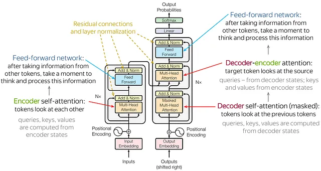
Transformers have revolutionized sequence modeling with their self-attention mechanism, which allows them to capture dependencies across entire sequences regardless of their length , this architecture has become the backbone of many state-of-the-art models in nlp and other domains due to its ability to model complex relationships between tokens in a sequence.
Transformers face challenges related to computational complexity and memory usage, especially as sequence lengths increase , the self-attention mechanism operates with quadratic complexity concerning sequence length, leading to significant resource requirements for very long sequences, despite these limitations Transformers remain a cornerstone of modern AI due to their flexibility and powerful performance in handling various types of data and tasks.
Transformer-Mamba Hybrid Architecture
The Transformer-Mamba hybrid architecture combines the best features of both Transformer and Mamba models to address their individual limitations , this hybrid approach leverages the Transformer’s self-attention mechanism to capture intricate long-range dependencies and Mamba’s efficient sequential processing to reduce computational and memory overhead , by integrating Mamba’s recurrent mechanisms with the Transformer’s self-attention, the hybrid model achieves a balance between modeling complex dependencies and maintaining resource efficiency , this combination allows for scalable, high-performance models that can handle both short-term and long-term dependencies effectively.
The Transformer-Mamba hybrid is particularly useful in scenarios where long sequences need to be processed efficiently without compromising on the model’s ability to understand complex relationships within the data.
Examples of Hybrid Architectures
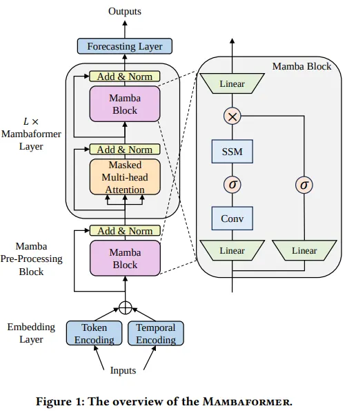
Mambaformer
Overview: Mambaformer integrates the self-attention mechanism of Transformers with the efficient sequential processing of Mamba , this hybrid model uses Mamba layers to handle long sequences efficiently while incorporating Transformer-like self-attention for capturing complex dependencies.
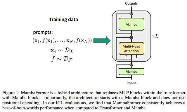
Performance: Mambaformer has shown improved performance in natural language processing tasks compared to traditional Transformers of similar size , it maintains high accuracy while reducing memory consumption and computational overhead, particularly for tasks involving very long sequences.
Jamba
Overview: Jamba combines the Transformer’s self-attention mechanism with Mamba’s recurrence-based approach , this hybrid architecture aims to harness the strengths of both models, allowing for efficient processing of long sequences with complex dependencies.
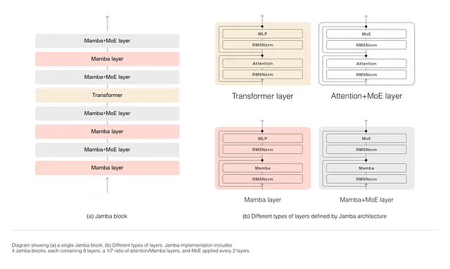
Performance: Jamba has demonstrated state-of-the-art results in various benchmarks, outperforming comparable models in terms of efficiency and accuracy , it achieves higher throughput and better handling of long sequences compared to pure Transformer models.
MambaVision
Overview: MambaVision blends Transformer components with Mamba’s efficient sequence handling, optimized for vision tasks , it utilizes self-attention for capturing global features and Mamba’s mechanisms for local feature extraction.
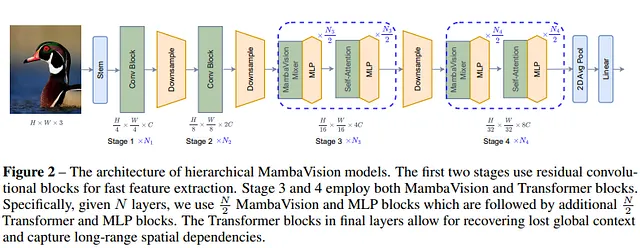
Performance: MambaVision has outperformed traditional CNNs and Transformer-based vision models in tasks such as image classification, object detection, and segmentation , it offers improved accuracy and efficiency in processing high-resolution images and complex visual data.
Hybrid Time Series Models
Overview: Hybrid models designed for time series forecasting combine Transformer’s ability to model long-term dependencies with Mamba’s efficiency in handling sequential data , these models use Transformer-like mechanisms for capturing complex patterns and Mamba’s recurrent features for efficient processing.
Performance: Hybrid time series models have achieved superior forecasting accuracy compared to traditional time series models , they balance the need for long-term dependency modeling with the efficiency required for processing large-scale data, resulting in better performance on both short-term and long-term forecasts.
In this project guide, we will create a custom hybrid architecture by integrating insights from our previous work on Mamba and Transformer-based models.
Code Time
Install Import essential dependencies
! pip install einops datasets
import torch
import math
import time
from einops import einsum, rearrange, repeat
import torch.nn.functional as F
from torch import Tensor, nn
from typing import Optional
from transformers import AutoTokenizer
from datasets import load_dataset
from torch.utils.data import Dataset, DataLoader
from tqdm import tqdm
Train The Tokenizer
We start by defining a function to get training data from a dataset of algerian darija , we use the load_dataset function to load the dataset and then yield chunks of 1000 text samples at a time.
Next we initialize a base tokenizer from a pre-trained Mamba model , after that, we train a new tokenizer using the chunks of training data with a specified vocabulary size , we then customize this tokenizer by setting its padding token to the end-of-sequence token and adding new special tokens related to FIM .
For these new tokens, we retrieve their token ids and optionally include a padding token id based on the truncate_or_pad flag.
# Function to get training data
def get_training_corpus():
    dataset = load_dataset("ayoubkirouane/Algerian-Darija", split="v1")
    for i in range(0, len(dataset), 1000):
        yield dataset[i : i + 1000]["Text"]

# Initialize the base tokenizer
base_tokenizer = AutoTokenizer.from_pretrained("state-spaces/mamba-130m-hf")

# Train the new tokenizer
new_tokenizer = base_tokenizer.train_new_from_iterator(get_training_corpus(), vocab_size=3000)


new_tokenizer.pad_token = new_tokenizer.eos_token

fim_prefix_token = "<fim_prefix>"
fim_middle_token = "<fim_middle_token>"
fim_suffix_token = "<fim_suffix_token>"
fim_pad_token = "<fim_pad>"

# Get the FIM-specific tokens and get their token ids
new_tokenizer.add_tokens(
    [
        fim_prefix_token,
        fim_middle_token,
        fim_middle_token,
        fim_pad_token,
    ]
)
prefix_tok_id = new_tokenizer.convert_tokens_to_ids(fim_prefix_token)
middle_tok_id = new_tokenizer.convert_tokens_to_ids(fim_middle_token)
suffix_tok_id = new_tokenizer.convert_tokens_to_ids(fim_middle_token)
pad_tok_id = None

fim_tokens = [prefix_tok_id, middle_tok_id, suffix_tok_id]


# If truncate_or_pad is on, also get pad token id
truncate_or_pad = True
if truncate_or_pad:
    pad_tok_id = new_tokenizer.convert_tokens_to_ids(fim_pad_token)
    fim_tokens.append(pad_tok_id)

# Save the new tokenizer
new_tokenizer.save_pretrained("new_tokenizer")
Finally we save the new tokenizer to a directory for future use. This approach ensures our tokenizer is well-suited for handling algerian darija text and any special requirements we might have
Multi-Head Attention Mechanism
In this MultiHeadAttention module, we start by initializing the layers for query, key, and value projections using linear transformations , this setup includes defining the number of heads and the dimensionality of each head, with an option for linear attention if needed , in the forward pass, we first compute the query, key, and value projections from the input tensor and reshape them to accommodate multiple attention heads , we then scale the queries and use scaled dot-product attention to compute the attention output (flash attention-2).
class MultiHeadAttention(nn.Module):
    def __init__(
        self,
        dim: int,
        heads: int,
        dim_head: int,
        dropout: float = 0.1,
        use_linear_attn: bool = False,
    ):
        super().__init__()
        self.dim = dim
        self.heads = heads
        self.dim_head = dim_head
        self.dropout = dropout
        self.use_linear_attn = use_linear_attn

        inner_dim = heads * dim_head
        self.scale = dim_head ** -0.5

        # Query, Key, and Value projection layers
        self.to_q = nn.Linear(dim, inner_dim, bias=False)
        self.to_k = nn.Linear(dim, inner_dim, bias=False)
        self.to_v = nn.Linear(dim, inner_dim, bias=False)

        self.to_out = nn.Sequential(
            nn.Linear(inner_dim, dim),
            nn.Dropout(dropout)
        )

    def forward(self, x: Tensor, mask: Optional[Tensor] = None) -> Tensor:
        b, n, d = x.shape

        q = self.to_q(x).reshape(b, n, self.heads, self.dim_head).transpose(1, 2)
        k = self.to_k(x).reshape(b, n, self.heads, self.dim_head).transpose(1, 2)
        v = self.to_v(x).reshape(b, n, self.heads, self.dim_head).transpose(1, 2)

        q *= self.scale


        attn_output = F.scaled_dot_product_attention(q, k, v, is_causal=True)

        out = attn_output.transpose(1, 2).reshape(b, n, -1)

        return self.to_out(out)
Finally, we reshape and pass the output through a linear layer followed by dropout to produce the final result .
Linear Attention
In this module we start by projecting the input tensor into query, key, and value representations using a single linear layer that combines all three projections.
These projections are then split and reshaped to support multi-head attention , each query is scaled and softmax-ed to obtain attention weights, which are used to compute the context by applying matrix multiplication between the queries and keys , the resulting context is then used to generate the output by applying it to the values.
class LinearAttention(nn.Module):
    def __init__(self, dim, *, heads=4, dim_head=64, dropout=0.0):
        super().__init__()
        inner_dim = heads * dim_head
        self.heads = heads
        self.scale = dim_head**-0.5

        self.to_qkv = nn.Linear(dim, inner_dim * 3, bias=False)
        self.to_out = nn.Sequential(
            nn.Linear(inner_dim, dim),
            nn.Dropout(dropout)
        )

    def forward(self, x, mask=None):
        h = self.heads
        # Get queries, keys, and values
        q, k, v = self.to_qkv(x).chunk(3, dim=-1)

        # Reshape for multi-head attention
        q = q.reshape(q.shape[0], q.shape[1], h, -1).transpose(1, 2)
        k = k.reshape(k.shape[0], k.shape[1], h, -1).transpose(1, 2)
        v = v.reshape(v.shape[0], v.shape[1], h, -1).transpose(1, 2)

        q *= self.scale
        q = F.softmax(q, dim=-1)
        k = F.softmax(k, dim=-2)

        if mask is not None:
            k = k.masked_fill(mask, float('-inf'))

        # Compute context and output
        context = torch.einsum('b h n d, b h n e -> b h d e', q, k)
        out = torch.einsum('b h d e, b h n d -> b h n e', context, v)

        # Reshape back to original dimensions and apply the final linear layer
        out = out.transpose(1, 2).reshape(x.shape[0], x.shape[1], -1)
        return self.to_out(out)
After computing the attention output, we reshape it back to the original dimensions and apply a final linear layer followed by dropout.
Mamba Block
In the MambaBlock class we define a sophisticated neural network block designed to leverage both convolutional and selective state space techniques.
We initialize the block with various parameters including the dimensionality of the input (dim), depth, state dimensions (d_state), and convolutional parameters , the in_proj layer projects the input into a higher-dimensional space, which is then processed through a 1D convolution to capture local patterns , the x_proj layer projects the input to produce components needed for the selective state space model (ssm), including parameters for Δ, B, and C.
class MambaBlock(nn.Module):
    def __init__(
        self,
        dim: int = None,
        depth: int = 5,
        d_state: int = 16,
        expand: int = 2,
        d_conv: int = 4,
        conv_bias: bool = True,
        bias: bool = False,
    ):
        """A single Mamba block, as described in Figure 3 in Section 3.4 in the Mamba paper [1]."""
        super().__init__()
        self.dim = dim
        self.depth = depth
        self.d_state = d_state
        self.expand = expand
        self.d_conv = d_conv
        self.conv_bias = conv_bias
        self.bias = bias

        # If dt_rank is not provided, set it to ceil(dim / d_state)
        dt_rank = math.ceil(self.dim / 16)
        self.dt_rank = dt_rank

        # If dim_inner is not provided, set it to dim * expand
        dim_inner = dim * expand
        self.dim_inner = dim_inner

        # If dim_inner is not provided, set it to dim * expand
        self.in_proj = nn.Linear(dim, dim_inner * 2, bias=bias)

        self.conv1d = nn.Conv1d(
            in_channels=dim_inner,
            out_channels=dim_inner,
            bias=conv_bias,
            kernel_size=d_conv,
            groups=dim_inner,
            padding=d_conv - 1,
        )

        # x_proj takes in `x` and outputs the input-specific Δ, B, C
        self.x_proj = nn.Linear(
            dim_inner, dt_rank + self.d_state * 2, bias=False
        )

        # dt_proj projects Δ from dt_rank to d_in
        self.dt_proj = nn.Linear(dt_rank, dim_inner, bias=True)

        A = repeat(torch.arange(1, self.d_state + 1), "n -> d n", d=dim_inner)
        self.A_log = nn.Parameter(torch.log(A))
        self.D = nn.Parameter(torch.ones(dim_inner))
        self.out_proj = nn.Linear(dim_inner, dim, bias=bias)

    def forward(self, x: Tensor):
        (b, l, d) = x.shape

        x_and_res = self.in_proj(x)  # shape (b, l, 2 * d_in)
        x_and_res = rearrange(x_and_res, "b l x -> b x l")
        (x, res) = x_and_res.split(
            split_size=[self.dim_inner, self.dim_inner], dim=1
        )

        x = self.conv1d(x)[:, :, :l]
        x = F.silu(x)

        y = self.ssm(x)

        y = y * F.silu(res)

        output = self.out_proj(rearrange(y, "b dim l -> b l dim"))

        return output

    def ssm(self, x: Tensor):

        (d_in, n) = self.A_log.shape

        A = -torch.exp(self.A_log.float())  # shape (d_in, n)
        D = self.D.float()

        x_dbl = rearrange(x, "b d l -> b l d")
        x_dbl = self.x_proj(x_dbl)  # (b, l, dt_rank + 2*n)

        (delta, B, C) = x_dbl.split(
            split_size=[self.dt_rank, n, n], dim=-1
        )  # delta: (b, l, dt_rank). B, C: (b, l, n)
        delta = F.softplus(self.dt_proj(delta))  # (b, l, d_in)

        y = self.selective_scan(
            x, delta, A, B, C, D
        )  # This is similar to run_SSM(A, B, C, u) in The Annotated S4 [2]

        return y

    def selective_scan(self, u, delta, A, B, C, D):

        (b, d_in, l) = u.shape
        n = A.shape[1]


        deltaA = torch.exp(einsum(delta, A, "b l d_in, d_in n -> b d_in l n"))
        deltaB_u = einsum(
            delta, B, u, "b l d_in, b l n, b d_in l -> b d_in l n"
        )

        # Perform selective scan (see scan_SSM() in The Annotated S4 [2])
        x = torch.zeros((b, d_in, n), device=next(self.parameters()).device)
        ys = []
        for i in range(l):
            x = deltaA[:, :, i] * x + deltaB_u[:, :, i]
            y = einsum(x, C[:, i, :], "b d_in n , b n -> b d_in")
            ys.append(y)
        y = torch.stack(ys, dim=2)  # (b d_in l)

        if D is not None:
            y = y + u * rearrange(D, "d_in -> d_in 1")

        return y
In the forward pass, we project and split the input into x and residual components , the convolutional layer processes x, which is then passed through the ssm , the ssm incorporates learned parameters to perform a selective scan, capturing complex sequential dependencies and the final output is obtained by projecting the result back to the original dimensionality.
The ssm method implements the core selective state space model, using the parameters A, D, B, and C to perform a selective scan over the input sequence.
Feed Forward
The initialization sets up the dimensions for input and output, the internal dimensional multiplier, dropout rate, and whether to use bias , we compute the internal dimension based on the input dimension multiplied by a given factor (mult) , the project_in sequential block first linearly projects the input to this internal dimension and applies the silu activation function.
class FeedForward(nn.Module):
    def __init__(
        self,
        dim: Optional[int] = None,
        dim_out: Optional[int] = None,
        mult: Optional[int] = 4,
        post_act_ln: Optional[bool] = False,
        dropout: Optional[float] = 0.0,
        no_bias: Optional[bool] = False,
        triton_kernels_on: bool = False,
    ):

        super().__init__()
        self.dim = dim
        self.dim_out = dim_out
        self.mult = mult
        self.post_act_ln = post_act_ln
        self.dropout = dropout
        self.no_bias = no_bias
        self.triton_kernels_on = triton_kernels_on

        inner_dim = int(dim * mult)
        dim_out = dim_out or dim  # Default to input dimension if not provided

        # Determine activation function
        activation = nn.SiLU()


        project_in = nn.Sequential(
                nn.Linear(dim, inner_dim, bias=not no_bias), activation
            )

        # Define feedforward network
        if post_act_ln:
            self.ff = nn.Sequential(
                project_in,
                nn.LayerNorm(inner_dim),
                nn.Dropout(dropout),
                nn.Linear(inner_dim, dim_out, bias=not no_bias),
            )
        else:
            self.ff = nn.Sequential(
                project_in,
                nn.Dropout(dropout),
                nn.Linear(inner_dim, dim_out, bias=not no_bias),
            )

    def forward(self, x):

        return self.ff(x)
The ff layer is constructed differently depending on whether post_act_ln is True, if it is the network includes a LayerNorm applied after activation and dropout, followed by another linear transformation to project to the output dimension , if post_act_ln is False the network omits LayerNorm and directly applies dropout before projecting to the output dimension.
In the forward method we simply pass the input through the defined ff sequential block, applying all transformations and activations in one go , this modular approach allows for flexibility in designing feedforward networks tailored to specific tasks or architectural needs.
RMSNorm
This class implements a normalization technique that scales input tensors to stabilize training , during initialization the class calculates a scaling factor as the inverse square root of the dimensionality (dim) and initializes a learnable parameter g, which scales the normalized output.
class RMSNorm(nn.Module):
    def __init__(self, dim: int):
        super().__init__()
        self.scale = dim ** (-0.5)
        self.g = nn.Parameter(torch.ones(dim))

    def forward(self, x: Tensor) -> Tensor:
        return F.normalize(x, dim=-1) * self.scale * self.g
In the forward pass the input tensor x is first normalized across the last dimension using F.normalize , this normalization standardizes the tensor, reducing its variance , then the normalized tensor is scaled by multiplying with the previously computed scale factor and the learnable parameter g , this operation helps in adjusting the output's magnitude while keeping the training stable.
TransformerBlock
Here we combine components of both traditional and linear attention mechanisms to build a versatile transformer block , we initialize first the block with parameters defining the dimensionality, number of attention heads, and whether to use linear attention , inside the constructor we set up the attention mechanism — either MultiHeadAttention or LinearAttention based on the use_linear_attn flag and a feedforward network (FeedForward) , we also include a layer normalization step (nn.LayerNorm) to stabilize training.
class TransformerBlock(nn.Module):
    def __init__(
        self,
        dim: int,
        heads: int,
        dim_head: int,
        dropout: float = 0.1,
        ff_mult: int = 4,
        use_linear_attn: bool = False,
        *args,
        **kwargs,
    ):
        super().__init__()
        self.dim = dim
        self.heads = heads
        self.dim_head = dim_head
        self.dropout = dropout
        self.ff_mult = ff_mult
        self.use_linear_attn = use_linear_attn

        self.attn = MultiHeadAttention(dim, heads, *args, **kwargs)

        # Linear Attention
        self.linear_attn = LinearAttention(
            dim=dim, heads=heads, dim_head=dim_head, dropout=dropout
        )

        self.ffn = FeedForward(dim, dim, ff_mult, *args, **kwargs)

        # Normalization
        self.norm = nn.LayerNorm(dim)

    def forward(self, x: Tensor) -> Tensor:
        """
        Performs a forward pass of the TransformerBlock.

        Args:
            x (Tensor): The input tensor.

        Returns:
            Tensor: The output tensor.

        """
        if self.use_linear_attn:
            x = self.linear_attn(x)
            x = self.norm(x)
            x = self.ffn(x)
        else:
            x, _, _ = self.attn(x)
            x = self.norm(x)
            x = self.ffn(x)

        return x
In the forward method we conditionally apply either the LinearAttention or MultiHeadAttention to the input tensor x, for linear attention the tensor is processed directly and then normalized, followed by the feedforward network , if traditional attention is used the tensor undergoes multi-head attention, normalization, and then the feedforward network , this design allows the block to leverage either attention mechanism as needed, providing flexibility and efficiency in sequence modeling.
Mamba-Transformer block
In this class we combine mamba and transformer architectures to build a sophisticated block for sequence processing.
To start the block is initialized with various parameters, including dimensions, the number of attention heads, and depths for both mamba and transformer components , the constructor sets up multiple layers for each component: mamba blocks, transformer blocks, and feedforward networks (FeedForward), which are all organized into nn.ModuleList for modularity.
class MambaTransformerblock(nn.Module):

    def __init__(
        self,
        dim: int,
        heads: int,
        depth: int,
        dim_head: int,
        dropout: float = 0.1,
        ff_mult: int = 4,
        d_state: int = None,
        transformer_depth: int = 1,
        mamba_depth: int = 1,
        use_linear_attn: bool = False,
        *args,
        **kwargs,
    ):
        super().__init__()
        self.dim = dim
        self.depth = depth
        self.dim_head = dim_head
        self.d_state = d_state
        self.dropout = dropout
        self.ff_mult = ff_mult
        self.d_state = d_state
        self.transformer_depth = transformer_depth
        self.mamba_depth = mamba_depth

        # Mamba, Transformer, and ffn blocks
        self.mamba_blocks = nn.ModuleList([
            MambaBlock(dim, mamba_depth, d_state, *args, **kwargs)
            for _ in range(mamba_depth)
        ])
        self.transformer_blocks = nn.ModuleList([
            TransformerBlock(
                dim,
                heads,
                dim_head,
                dropout,
                ff_mult,
                use_linear_attn,
                *args,
                **kwargs,
            ) for _ in range(transformer_depth)
        ])

        self.ffn_blocks = nn.ModuleList([
            FeedForward(dim, dim, ff_mult, *args, **kwargs)
            for _ in range(depth)
        ])

        # Layernorm
        self.norm = nn.LayerNorm(dim)

    def forward(self, x: Tensor) -> Tensor:
        for mamba, attn, ffn in zip(
            self.mamba_blocks,
            self.transformer_blocks,
            self.ffn_blocks,
        ):
            x = self.norm(x)
            x = mamba(x) + x
            x = self.norm(x)
            x = attn(x) + x
            x = self.norm(x)
            x = ffn(x) + x

        return x
During the forward pass the input tensor x is sequentially processed through each mamba block, transformer block, and feedforward network.
Each mamba block enhances the tensor, which is then passed through a transformer block , after each block layer normalization is applied to stabilize training and improve convergence , the results from each block are added back to the input tensor, implementing a residual connection that helps in training deeper networks.
This hybrid approach integrates the strengths of mamba’s efficient sequence processing with transformer’s powerful attention mechanisms, followed by feedforward layers, to enhance the model’s capability in handling complex sequence tasks.
Mamba-Transformer
This class defines a model that integrates both mamba and transformer blocks designed for sequence processing tasks.
In the initialization, the model sets up several key components: an embedding layer to convert token indices into dense vectors, a hybrid MambaTransformerBlock to process these embeddings, and a final layer to produce logits , the MambaTransformerBlock combines mamba and transformer blocks, providing a rich representation of the input sequences.
class MambaTransformer(nn.Module):
    def __init__(
        self,
        num_tokens: int,
        dim: int,
        heads: int,
        depth: int,
        dim_head: int,
        dropout: float = 0.1,
        ff_mult: int = 4,
        d_state: int = None,
        return_embeddings: bool = False,
        transformer_depth: int = 1,
        mamba_depth: int = 1,
        use_linear_attn=False,
        *args,
        **kwargs,
    ):
        super().__init__()
        self.dim = dim
        self.depth = depth
        self.dim_head = dim_head
        self.d_state = d_state
        self.dropout = dropout
        self.ff_mult = ff_mult
        self.d_state = d_state
        self.return_embeddings = return_embeddings
        self.transformer_depth = transformer_depth
        self.mamba_depth = mamba_depth

        self.emb = nn.Embedding(num_tokens, dim)
        self.mt_block = MambaTransformerblock(
            dim,
            heads,
            depth,
            dim_head,
            dropout,
            ff_mult,
            d_state,
            return_embeddings,
            transformer_depth,
            mamba_depth,
            use_linear_attn,
            *args,
            **kwargs,
        )
        self.to_logits = nn.Sequential(
            RMSNorm(dim), nn.Linear(dim, num_tokens)
        )

    def forward(self, x: Tensor) -> Tensor:
        """
        Forward pass of the MambaTransformer model.

        Args:
            x (Tensor): Input tensor of shape (batch_size, sequence_length).

        Returns:
            Tensor: Output tensor of shape (batch_size, sequence_length, num_tokens).
        """
        x = self.emb(x)
        x = self.mt_block(x)

        if self.return_embeddings:
            return x

        else:
            return self.to_logits(x)
In the forward pass the input tensor xrepresenting token indices is first embedded into dense vectors. , these embeddings are then processed by the MambaTransformerBlock, which applies the hybrid sequence processing techniques, depending on the return_embeddings flag the model either returns the processed embeddings or further applies a RMSNorm layer followed by a linear transformation to generate logits for each token position, typically used for prediction tasks.
Create The Model
We create an instance of the MambaTransformer model , this model is configured to use the vocabulary size from new_tokenizer, a model dimension of 512, 16 attention heads, and a depth of 8 transformer layers and 8 mamba layers , it incorporates both mamba and transformer blocks, with each block having a dimension of 128 for attention heads and a state dimension of 512.
# Create an instance of the MambaTransformer model
model = MambaTransformer(
    num_tokens=new_tokenizer.vocab_size,  # Number of tokens in the input sequence
    dim=512,  # Dimension of the model
    heads=16,  # Number of attention heads
    depth=8,  # Number of transformer layers
    dim_head=128,  # Dimension of each attention head
    d_state=512,  # Dimension of the state
    dropout=0.1,  # Dropout rate
    ff_mult=4,  # Multiplier for the feed-forward layer dimension
    return_embeddings=False,  # Whether to return the embeddings,
    transformer_depth=8,  # Number of transformer blocks
    mamba_depth=8,  # Number of Mamba blocks,
    use_linear_attn=True,  # Whether to use linear attention
)
The dropout rate is set to 0.1, the feed-forward layer uses a multiplier of 4, and the model is configured to use linear attention, return_embeddings is set to False indicating that the model will output logits rather than embeddings.
This configuration specifies a substantial model architecture capable of handling complex sequence tasks with a balanced approach between attention mechanisms and feed-forward processing.
Dataset class
In this class we define a custom dataset class TextDataset for use with pytorch's DataLoader , the __init__ method initializes the dataset by loading it with the specified dataset_name and split, and sets up the tokenizer and maximum sequence length , the __len__ method return the length of the dataset.
class TextDataset(Dataset):
    def __init__(self, dataset_name, split, tokenizer, max_length):
        self.tokenizer = tokenizer
        self.max_length = max_length
        self.dataset = load_dataset(dataset_name, split=split)

    def __len__(self):
        return len(self.dataset)

    def __getitem__(self, idx):
        text = self.dataset[idx]['Text']  # Adjust 'text' if your dataset uses a different column name
        encoding = self.tokenizer(text, truncation=True,
                                  padding='max_length',
                                  max_length=self.max_length,
                                  return_tensors='pt') # Ensure PyTorch Tensor output

        input_ids = encoding['input_ids'].squeeze()

        # Assuming you want to use the input_ids as labels for language modeling

        # Shift labels
        labels = input_ids.clone()

        labels[:-1] = input_ids[1:]  # Shift labels
        return input_ids, labels  # Return both input_ids and labels
__getitem__ method retrieves a text sample by its index, tokenizes it while applying truncation and padding to ensure each sequence is of max_length , it then prepares the input ids and creates labels for language modeling by shifting the input ids one position forward the method in the end returns both the input_ids and labels as pytorch tensors.
Create the Trainer
The train function orchestrates the training of a MambaTransformer model, managing both the training and evaluation processes , it initializes the model, optimizer, and optional learning rate scheduler, then iterates over the training dataset for a specified number of epochs.
During training it performs forward passes, computes and backpropagates losses, and updates the model weights, incorporating gradient clipping to prevent instability.
def train(model: MambaTransformer,
          train_data: DataLoader,
          optimizer: torch.optim.Optimizer,

          val_data: DataLoader = None,
          epochs: int = 10,
          tokenizer: AutoTokenizer = new_tokenizer,
          device: str = 'cuda' if torch.cuda.is_available() else 'cpu',
          clip_grad_norm: float = 1.0,
          lr_scheduler=None):
    """Trains the Mistral model.

    Args:
        model: The Mistral model to train.
        train_data: A DataLoader for the training dataset.
        optimizer: The optimizer to use for training.
        epochs: The number of training epochs.
        device: The device to use for training (e.g., 'cuda' or 'cpu').
        clip_grad_norm: The maximum norm of the gradients to clip.
        lr_scheduler: An optional learning rate scheduler.
    """

    model = model.to(device)
    model.train()

    print("Training...")
    for epoch in range(epochs):
        print(f"Epoch {epoch+1}/{epochs}")
        total_loss = 0.0
        start_time = time.time()

        for batch in tqdm(train_data, leave=False):
            input_ids, labels = batch

            input_ids, labels = input_ids.to(device), labels.to(device)

            optimizer.zero_grad()

            # Forward pass
            outputs = model(input_ids)

            # Calculate loss (use cross-entropy loss for language modeling)
            loss_fn = nn.CrossEntropyLoss()
            loss = loss_fn(outputs.view(-1, tokenizer.vocab_size), labels.view(-1))

            # Backward pass
            loss.backward()

            # Clip gradients
            torch.nn.utils.clip_grad_norm_(model.parameters(), clip_grad_norm)

            # Update weights
            optimizer.step()

            if lr_scheduler is not None:
                lr_scheduler.step()

            total_loss += loss.item()


        avg_loss = total_loss / len(train_data)
        elapsed_time = time.time() - start_time
        print(f"Average loss: {avg_loss:.4f} | Elapsed time: {elapsed_time:.2f}s")

        if val_data is not None:
          # Evaluation Phase
          model.eval()
          eval_loss = 0
          with torch.no_grad():
              for step, batch in enumerate(val_data):
                  # Get input_ids and labels from the batch
                  input_ids, labels = batch
                  input_ids = input_ids.to(device)  # Send input_ids to the device
                  labels = labels.to(device)  # Send labels to the device

                  # Forward pass
                  outputs = model(input_ids)

                  # Calculate loss
                  loss = F.cross_entropy(outputs.view(-1, tokenizer.vocab_size), labels.view(-1), ignore_index=tokenizer.pad_token_id)
                  eval_loss += loss.item()
          avg_eval_loss = eval_loss / len(val_data)
          print(f"Epoch: {epoch+1}, Evaluation Loss: {avg_eval_loss:.4f}")
    model_save_path = "Hybrid.pt"
    torch.save(model.state_dict(), model_save_path)
    print("Training complete!")
If a validation dataset is provided it evaluates the model’s performance at the end of each epoch computing and printing the validation loss , the function also includes functionality to save the trained model to a file, ensuring that the learned parameters can be reused or deployed later.
well it is a basic routine for effectively training and evaluating the model, with attention to important aspects like gradient clipping and performance tracking.
Optimizer: torch.optim.AdamW is used with a learning rate of 1e-4 for the model parameters , this optimizer is well-suited for handling the weight updates during training.
optimizer = torch.optim.AdamW(model.parameters(), lr=1e-4)
lr_scheduler = torch.optim.lr_scheduler.ReduceLROnPlateau(optimizer, 'min', patience=3)
Learning Rate Scheduler: torch.optim.lr_scheduler.CosineAnnealingLR adjusts the learning rate using a cosine annealing schedule, with a maximum number of iterations (T_max) set to 10 , this scheduler gradually reduces the learning rate following a cosine curve, helping the model converge smoothly towards the end of training.
train_dataset = TextDataset("ayoubkirouane/Algerian-Darija",
                      "v1",
                      new_tokenizer,
                      max_length=128)
train_loader = DataLoader(train_dataset, batch_size=4, shuffle=False)
Dataset: TextDataset is initialized with the ayoubkirouane/Algerian-Darija dataset from the datasets library, using the v1 split , it utilizes new_tokenizer for tokenization with a maximum sequence length of 128 tokens.
DataLoader: DataLoader is created with the train_dataset for batching. It uses a batch size of 4 and does not shuffle the data (shuffle=False) , this setup allows for efficient data loading during training, with each batch containing 4 samples.
Start The Training
train(model=model ,
      train_data=train_loader,
      optimizer=optimizer,
      tokenizer=new_tokenizer,
      epochs=1,
      clip_grad_norm=1.0,
      lr_scheduler=lr_scheduler)
This will start the training loop and print the progress and average loss for the specified number of epochs.
Generate Text
- Perform a forward pass through the model.
- Extract logits for the last token position and apply softmax to get probabilities.
- Select the top 50 probable tokens and sample from them.
- Append the sampled token to the sequence.
device = torch.device("cuda" if torch.cuda.is_available() else "cpu")

max_length = 30
num_return_sequences = 10


tokens = new_tokenizer.encode("نتا  ")
tokens = torch.tensor(tokens , dtype=torch.long)
tokens = tokens.unsqueeze(0).repeat(num_return_sequences, 1)

x = tokens.to(device)

while x.size(1) < max_length:

    with torch.no_grad():
        outputs = model(x)
        logits = outputs[0] if isinstance(outputs, tuple) else outputs
        logits = logits[:, -1, :]
        probs = F.softmax(logits, dim=-1)
        topk_probs, topk_indices = torch.topk(probs, 50, dim=-1)

        ix = torch.multinomial(topk_probs, 1)
        xcol = torch.gather(topk_indices, -1, ix)
        x = torch.cat((x, xcol), dim=1)

# print the generated text
for i in range(num_return_sequences):
    tokens = x[i, :max_length].tolist()
    decoded = new_tokenizer.decode(tokens, skip_special_tokens=True)
    print(">", decoded)
This code is designed to generate text using the trained MambaTransformer model , it initializes tokens, processes them through the model to generate sequences, and prints the decoded results.