Mistral 7B Model

Mistral 7B is a 7 billion parameter language model designed for superior performance and efficiency.

This report provides a detailed analysis of its architectural innovations, focusing on the key components that contribute to its high performance and efficient inference:

Mistral Architecture

Mistral 7B is based on the standard transformer architecture (Decoder-only), employing a multi-headed self-attention mechanism to capture complex dependencies within the input sequence.

Key parameters of the architecture are:

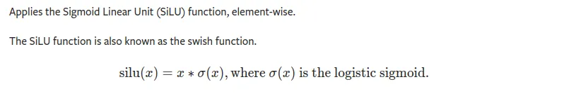
• n_layers: 32 (number of transformer layers)
• head_dim: 128 (dimension of each attention head)
• hidden_dim: 14336 (dimension of the feed-forward network)
• dim: 4096 (embedding dimension)
• n_heads: 32 (number of attention heads)
• n_kv_heads: 8 (number of attention heads for key/value pairs)
• window_size: 4096 (maximum number of tokens attended to by each token)
• context_len: 8192 (maximum sequence length)
• vocab_size: 32000 (vocabulary size)
• Activation Function: The silu (Sigmoid Linear Unit) activation function helps the model decide which information is relevant during processing.
• Sliding Window: A sliding_window size of 4096 allows the model to efficiently process large chunks of data by focusing on this fixed-size window of the most recent tokens.
• Rope Theta: The rope_theta parameter set to 10000.0 is a technical detail related to the model's positional encoding mechanism.

Sliding Window Attention (SWA)

Sliding Window Attention (SWA) is a novel approach to handling long sequences of text , traditional attention mechanisms in transformers require quadratic memory and computation costs with respect to the input sequence length. This becomes impractical for very long texts. SWA addresses this issue by breaking the input sequence into overlapping windows and computing self-attention within each window separately.

The overlapping windows ensure that information can flow across the entire sequence, even though attention is only computed locally within each window. this method significantly reduces memory usage and computational requirements, enabling the model to process longer texts more efficiently. by focusing on smaller, manageable chunks of text at a time, SWA maintains the ability to capture long-range dependencies without the prohibitive resource costs of traditional attention mechanisms.

Rolling Buffer Cache

The Rolling Buffer Cache is another key innovation in Mistral 7b, designed to optimize memory usage and processing speed for long text sequences. in essence, it acts as a dynamic memory buffer that retains useful information across sliding windows.

When processing a sequence with SWA, the Rolling Buffer Cache stores intermediate representations from previous windows, as the sliding window moves along the sequence, the cache updates by discarding obsolete data and incorporating new information , this approach minimizes redundant computations and reduces the memory footprint, as only a subset of the sequence’s data is actively processed and stored at any given time.

The Rolling Buffer Cache is particularly advantageous in scenarios where the context of earlier parts of the text is relevant to later parts, by maintaining a continuous flow of information and efficiently managing memory resources, it enhances the model’s ability to handle extensive texts seamlessly.

Pre-fill and Chunking

Pre-fill and Chunking is a strategy that further optimizes the processing of long sequences in Mistral 7b, this technique involves pre-processing the input text into smaller, fixed-size chunks before feeding them into the model, each chunk is processed independently, which allows for parallelization and reduces the complexity of handling the entire sequence at once.

Pre-fill refers to the process of initializing the model with a pre-defined context or state before processing each chunk, this initialization helps the model retain relevant information from previous chunks, ensuring coherence and continuity across the entire sequence, by dividing the input into manageable chunks and pre-filling the model with contextual information, this method mitigates the issues associated with processing long sequences in one go.

Chunking not only improves computational efficiency but also enhances the model’s performance by ensuring that each part of the sequence is attended to appropriately, it strikes a balance between granularity and context, enabling Mistral to process long texts effectively without overwhelming the model with excessive computational demands.

Rotary Position Embedding (RoPE)

Rotary Position Embedding (RoPE) is a technique used to encode positional information in transformer models, it was introduced in the paper “RoFormer: Enhanced Transformer with Rotary Position Embedding” .

How It Works:

• Traditional Position Embeddings: In standard transformers, position embeddings are added to token embeddings to provide information about the position of each token in the sequence.

• RoPE: RoPE modifies this approach by encoding positional information through a rotation mechanism. Instead of adding position embeddings, RoPE applies a rotary transformation to the attention mechanism, which helps the model learn relative positions of tokens more effectively. Key Concepts:

• Rotation Mechanism: RoPE uses complex-valued representations and applies a rotation operation based on the position of tokens. This rotation adjusts the attention mechanism so that it takes into account the relative positions of tokens.

• Relative Position Awareness: By incorporating relative positional information, RoPE helps the model understand how far apart tokens are from each other, which can be beneficial for capturing long-range dependencies in sequences.

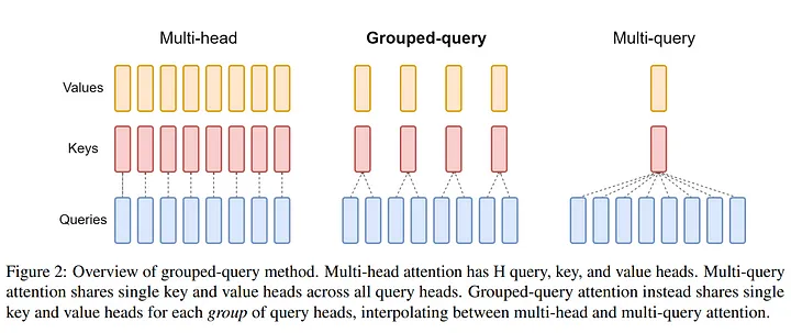
Grouped-Query Attention (GQA)

Grouped-Query Attention (GQA) is a technique for improving the efficiency and effectiveness of the attention mechanism in transformer models. It was introduced in the paper “GQA: Training Generalized Multi-Query Transformer Models from Multi-Head Checkpoints” .

How It Works:

• Traditional Multi-Head Attention: In traditional multi-head attention, multiple attention heads compute attention over the entire sequence, which can be computationally expensive.

• GQA: GQA modifies the attention mechanism by grouping queries and computing attention in a more structured and efficient manner.

Key Concepts:

• Query Grouping: GQA divides queries into groups and processes them in parallel. Each group focuses on different parts of the attention mechanism, allowing the model to capture a diverse range of features.
• Efficient Attention Computation: By grouping queries, GQA reduces the computational complexity of attention operations, leading to faster and more efficient processing.

---

We’ve walked through some pretty cool concepts like sliding Window attention, rolling buffer cache, and grouped-query attention. Now it’s time to see these ideas in action .

In the next section, we’ll take everything we’ve learned about the Mistral 7B architecture and put it into practice, get ready for the “Code Time” where we’ll dive into the actual implementation details and start building the model together.

This is where things get exciting, so let’s roll up our sleeves and bring these concepts to life!

---

Code Time

Here we’re getting everything we need to start building and training our model. We’re importing some essential tools from libraries that help us handle the heavy lifting of AI development.

import torch
from torch import nn
from torch.nn import functional as F
from typing import Tuple, Optional
import math
from datasets import load_dataset
from transformers import AutoTokenizer
from torch.utils.data import DataLoader, Dataset
from transformers import get_linear_schedule_with_warmup

Setting Up Model Configuration

In this section, we’re setting up the ModelArgs class, which acts like a blueprint for our model. Think of it as a detailed plan that specifies how our model should be built and what it should look like.

class ModelArgs:
    def __init__(
        self,
        dim: int,
        n_layers: int,
        head_dim: int,
        hidden_dim: int,
        n_heads: int,
        n_kv_heads: int,
        norm_eps: float,
        vocab_size: int,
        rope_theta: float = 10000,
    ):
        self.dim = dim
        self.n_layers = n_layers
        self.head_dim = head_dim
        self.hidden_dim = hidden_dim
        self.n_heads = n_heads
        self.n_kv_heads = n_kv_heads
        self.norm_eps = norm_eps
        self.vocab_size = vocab_size
        self.rope_theta = rope_theta

Implementing RMSNorm for Normalization

We’re defining here the RMSNorm class, which plays a crucial role in stabilizing our model’s training process.

class RMSNorm(nn.Module):
    def __init__(self, dims: int, eps: float = 1e-5):
        super().__init__()
        self.weight = nn.Parameter(torch.ones(dims))
        self.eps = eps

    def _norm(self, x):
        return x * (x.square().mean(-1, keepdim=True) + self.eps).rsqrt()

    def forward(self, x):
        output = self._norm(x.float()).type(x.dtype)
        return self.weight * output

• dims: this parameter specifies the number of dimensions we’re working with in the model. It sets up the scale for our normalization process.
• eps: this is a tiny value we add to avoid any potential calculation issues. It’s like a safety net to ensure our calculations remain stable.

Implementing Feed Forward Network

The FeedForward class is responsible for transforming the data as it moves through the model. It applies a series of linear transformations to process and enhance the information. Think of it as the model’s way of refining and expanding on the data it receives.

class FeedForward(nn.Module):
    def __init__(self, args: "ModelArgs"):
        super().__init__()

        self.w1 = nn.Linear(args.dim, args.hidden_dim, bias=False)
        self.w2 = nn.Linear(args.hidden_dim, args.dim, bias=False)
        self.w3 = nn.Linear(args.dim, args.hidden_dim, bias=False)

    def forward(self, x) -> torch.Tensor:
        return self.w2(F.silu(self.w1(x)) * self.w3(x))

We define three linear layers : w1, w2, and w3 which are like different stages of processing for the data:

• w1: takes the input data and projects it to a higher-dimensional space. this helps the model learn more complex patterns.
• w2: applies a non-linear activation function, Silu, which introduces non-linearity into the model. non-linearity is crucial for the model to learn complex relationships.

w3: Combines the output from w1 with the original input data to refine and produce the final result.

ROPE

RoPE is a technique we covered earlier in the blog, where we explored how positional encodings help the model understand the order of words in a sequence.

class RoPE(nn.Module):
    def __init__(self, dim: int, traditional: bool = False, base: float = 10000.0):
        super().__init__()
        self.dim = dim
        self.traditional = traditional
        self.base = base
        self.freqs = self.create_freqs(dim // 2)

    def create_freqs(self, n: int):
        freqs = 1.0 / (self.base ** (torch.arange(0, n, 2) / n))
        return freqs

    def forward(self, x: torch.Tensor, offset: int = 0):
        if self.traditional:
            t = torch.arange(x.shape[2], device=x.device) + offset
        else:
            t = torch.arange(x.shape[2], device=x.device)
        freqs = self.freqs.to(x.device)
        t_sin = torch.sin(t[:, None] * freqs[None, :])
        t_cos = torch.cos(t[:, None] * freqs[None, :])
        return torch.stack([x[..., 0::2] * t_cos + x[..., 1::2] * t_sin,
                           x[..., 0::2] * t_sin - x[..., 1::2] * t_cos], dim=-1).flatten(-2, -1)

RoPE creates a set of frequencies that represent different positions in the sequence of words. these frequencies help encode where each word is located in the sequence.

So this class applies these frequencies to the input data by calculating sine and cosine values. this is a sophisticated way to add information about word positions into the model. it’s like adding a timestamp to each word to tell the model where it is in the sentence .

Implementing Attention (GQA, RBC)

In this Attention class, we bring to life several techniques we discussed earlier, including Grouped-Query Attention (GQA), and Rolling Buffer Cache , here’s a look at how these concepts are applied in the code.

Initialization: We set up the attention mechanisms by defining the number of attention heads and the size of the key and value vectors. We also initialize the Rotary Position Embedding (RoPE) class, which we covered before for enhancing the positional information in our attention mechanism.

class Attention(nn.Module):
    def __init__(self, args: "ModelArgs"):
        super().__init__()
        self.args = args

        self.n_heads: int = args.n_heads
        self.n_kv_heads: int = args.n_kv_heads

        self.repeats = self.n_heads // self.n_kv_heads

        self.scale = self.args.head_dim**-0.5

        self.wq = nn.Linear(args.dim, args.n_heads * args.head_dim, bias=False)
        self.wk = nn.Linear(args.dim, args.n_kv_heads * args.head_dim, bias=False)
        self.wv = nn.Linear(args.dim, args.n_kv_heads * args.head_dim, bias=False)
        self.wo = nn.Linear(args.n_heads * args.head_dim, args.dim, bias=False)
        self.rope = RoPE(args.head_dim, traditional=True, base=args.rope_theta)

    def forward(
        self,
        x: torch.Tensor,
        mask: Optional[torch.Tensor] = None,
        cache: Optional[Tuple[torch.Tensor, torch.Tensor]] = None,
    ) -> torch.Tensor:
        B, L, D = x.shape

        queries, keys, values = self.wq(x), self.wk(x), self.wv(x)

        # Prepare the queries, keys and values for the attention computation
        queries = queries.view(B, L, self.n_heads, -1).transpose(1, 2)
        keys = keys.view(B, L, self.n_kv_heads, -1).transpose(1, 2)
        values = values.view(B, L, self.n_kv_heads, -1).transpose(1, 2)

        def repeat(a):
            a = torch.cat([a.unsqueeze(2)] * self.repeats, dim=2)
            return a.view([B, self.n_heads, L, -1])

        keys, values = map(repeat, (keys, values))

        # Rolling Buffer Cache
        if cache is not None:
            key_cache, value_cache = cache
            queries = self.rope(queries, offset=key_cache.shape[2])
            keys = self.rope(keys, offset=key_cache.shape[2])
            keys = torch.cat([key_cache, keys], dim=2)
            values = torch.cat([value_cache, values], dim=2)
        else:
            queries = self.rope(queries)
            keys = self.rope(keys)

        scores = (queries * self.scale) @ keys.transpose(-1, -2)
        if mask is not None:
            scores += mask
        scores = F.softmax(scores.float(), dim=-1).type(scores.dtype)
        output = (scores @ values).transpose(1, 2).contiguous().view(B, L, -1)
        return self.wo(output), (keys, values)

Grouped-Query Attention (GQA): Attention class applies GQA by organizing the queries into different groups based on their attention heads and using a repeated key and value approach. this organization allows for efficient processing and better management of attention across different segments of the input.

Rolling Buffer Cache: We implement the Rolling Buffer Cache technique by handling the cache parameter. when cache is used, it helps manage past attention computations and maintains context over long sequences, which aligns with the Rolling Buffer Cache approach we discussed.

Implementing TransformerBlock

In the TransformerBlock class, we see the application of multiple techniques that we’ve explored in our earlier sections.

class TransformerBlock(nn.Module):
    def __init__(self, args: "ModelArgs"):
        super().__init__()
        self.n_heads = args.n_heads
        self.dim = args.dim
        self.attention = Attention(args)
        self.feed_forward = FeedForward(args=args)
        self.attention_norm = RMSNorm(args.dim, eps=args.norm_eps)
        self.ffn_norm = RMSNorm(args.dim, eps=args.norm_eps)
        self.args = args

    def forward(
        self,
        x: torch.Tensor,
        mask: Optional[torch.Tensor] = None,
        cache: Optional[Tuple[torch.Tensor, torch.Tensor]] = None,
    ) -> torch.Tensor:
        r, cache = self.attention(self.attention_norm(x), mask, cache)
        h = x + r
        r = self.feed_forward(self.ffn_norm(h))
        out = h + r
        return out, cache

We combine attention mechanisms with feed-forward networks to create the core building block of our model .

• Attention Mechanism: we use the Attention class here, which integrates Sliding Window Attention (SWA), Grouped-Query Attention (GQA), and Rolling Buffer Cache. this part of the block is responsible for capturing the relationships between different parts of the input sequence.
• Layer Normalization with RMSNorm: both the attention output and the feed-forward output are normalized using RMSNorm, which we talked about earlier for stabilizing training and improving performance.
• Feed-Forward Network: after attention, we process the data through a Feed-Forward Network to further refine the information, this is done using the FeedForward class we defined before, which applies linear transformations with a non-linearity in between.
• Residual Connections: the block uses residual connections to add the original input to the output of the attention and feed-forward steps, this technique helps the model learn more effectively by allowing gradients to flow more easily through the network.

Implementing Mistral

The Mistral class is where we bring together all the components we’ve been working on to build the full model, this class defines the structure of the Mistral 7B model and how it processes input data.

class Mistral(nn.Module):
    def __init__(self, args: "ModelArgs"):
        super().__init__()
        self.args = args
        self.vocab_size = args.vocab_size
        self.n_layers = args.n_layers
        assert self.vocab_size > 0
        self.tok_embeddings = nn.Embedding(args.vocab_size, args.dim)
        self.layers = nn.ModuleList([TransformerBlock(args=args) for _ in range(args.n_layers)])
        self.norm = RMSNorm(args.dim, eps=args.norm_eps)
        self.output = nn.Linear(args.dim, args.vocab_size, bias=False)
        self.apply(self._init_weights)

    def _init_weights(self, module):
        if isinstance(module, nn.Linear):
            nn.init.xavier_uniform_(module.weight)
            if module.bias is not None:
                nn.init.zeros_(module.bias)
        elif isinstance(module, nn.Embedding):
            nn.init.xavier_uniform_(module.weight)
        elif isinstance(module, RMSNorm):
            nn.init.ones_(module.weight)
        elif isinstance(module, nn.MultiheadAttention):
            nn.init.xavier_uniform_(module.in_proj_weight)
            if module.in_proj_bias is not None:
                nn.init.zeros_(module.in_proj_bias)
            nn.init.xavier_uniform_(module.out_proj.weight)
            if module.out_proj.bias is not None:
                nn.init.zeros_(module.out_proj.bias)

    def _generate_square_subsequent_mask(self, sz):
        mask = torch.triu(torch.ones(sz, sz) * float('-inf'), diagonal=1)
        return mask

    def forward(
        self,
        inputs: torch.Tensor,
        cache=None,
    ):
        h = self.tok_embeddings(inputs)

        mask = None
        if h.shape[1] > 1:
            mask = self._generate_square_subsequent_mask(h.shape[1]).to(h.device)

        if cache is None:
            cache = [None] * len(self.layers)

        for e, layer in enumerate(self.layers):
            h, cache[e] = layer(h, mask, cache[e])

        return self.output(self.norm(h)), cache

1 . Token Embeddings: we start by creating token embeddings with nn.Embeddingthis layer converts input tokens into dense vectors of a fixed size , this is our starting point for processing language data.

2 . Transformer Blocks: we assemble a stack of TransformerBlock layers, which are the building blocks of our model , these blocks use the attention mechanisms, feed-forward networks, and normalization techniques that we’ve discussed, this stack of layers processes the input data through multiple stages of attention and transformation.

3 . Normalization and Output Layer: after processing through the transformer blocks, the data is normalized with RMSNorm and passed through a Linear layer to produce the final output logits , this step is crucial for stabilizing training and generating predictions.

4 . Weight Initialization: we use a custom weight initialization function to set up the model parameters , this function ensures that the layers start with appropriate values to support effective learning ( you can start from existing checkpoint )

5 . Mask Generation: for training, we generate a mask to ensure that the model only attends to previous tokens in the sequence, preserving the autoregressive nature of the model , this concept was touched upon in our discussion of SWA and GQA techniques.

6 . Forward Pass: in the forward method, we pass the input tokens through the embeddings, apply the transformer layers, and generate the output predictions, this method also manages caching for efficient processing of long sequences, a concept we’ve explored under Rolling Buffer Cache.

Initializing the Model

We define a ModelArgs object with specific values for various hyperparameters of the Mistral model.

model_args = ModelArgs(
    dim=4096,             # Embedding dimension
    n_layers=32,          # Number of Transformer layers
    head_dim=128,         # Head dimension for multi-head attention
    hidden_dim=14336,     # Dimension of hidden layer in the feedforward network
    n_heads=32,           # Number of attention heads
    n_kv_heads=32,        # Number of key/value heads (can be different from n_heads)
    norm_eps=1e-5,        # Epsilon value for normalization
    vocab_size=32000,     # Size of your vocabulary
    rope_theta=10000,     # Base value for Rotary Position Embeddings
)

# Create the Mistral model
model = Mistral(model_args)

Each parameter plays a key role in shaping how the model processes data:

Training the tokenizer

In this section, we’ll go through the process of creating and testing a new tokenizer , this is a crucial step for customizing our model to better handle specific text data, like Algerian Darija in our case, we’ll cover how to set up the tokenizer, train it, and verify that it’s working as expected.

# Function to get training data
def get_training_corpus():
    dataset = load_dataset("text", data_files={"train": "/content/cleaned_data.txt"})
    for i in range(0, len(dataset["train"]), 1000):
        yield dataset["train"][i : i + 1000]["text"]


# Load the base tokenizer
base_tokenizer = AutoTokenizer.from_pretrained("unsloth/mistral-7b-v0.3-bnb-4bit")

# Train the new tokenizer
new_tokenizer = base_tokenizer.train_new_from_iterator(get_training_corpus(), 
               vocab_size=1000) # increase the vocab_size to match your need

# Save the new tokenizer
new_tokenizer.save_pretrained("new_tokenizer")

# Test the new tokenizer
test_text = "الهجرة كلمة تسمعها بزاف في بلاديء أنا عمري ماخممت فيها"
encoded = new_tokenizer.encode(test_text)
decoded = new_tokenizer.decode(encoded)

print(f"Encoded: {encoded}")
print(f"Decoded: {decoded}")

We start by defining a function to prepare our text data for the tokenizer , next, we load the base tokenizer from a pre-trained model here we are loading the AutoTokenizer for the Mistral-7B-v0.3 model from Hugging Face’s model hub (extended vocabulary to 32768) , this pre-trained tokenizer provides a starting point for our new tokenizer, it includes a basic vocabulary and tokenization rules that we will extend and refine with our specific data , we then train the new tokenizer on our text dat , after training, we save the new tokenizer to disk (you can test it if you want).

Setting up the Dataset Class

In this section, we are defining a custom dataset class for handling text data, which is a crucial step for preparing our data for training. Let’s break down what this class does and why we designed it this way.

class TextDataset(Dataset):
    def __init__(self, file_path, tokenizer, max_length):
        self.tokenizer = tokenizer
        self.max_length = max_length
        with open(file_path, 'r', encoding='utf-8') as f:
            self.texts = f.readlines()

    def __len__(self):
        return len(self.texts)

    def __getitem__(self, idx):
        text = self.texts[idx]
        encoding = self.tokenizer(text, truncation=True,
                                  padding='max_length',
                                  max_length=self.max_length,
                                  return_tensors='pt') # Ensure PyTorch Tensor output

        input_ids = encoding['input_ids'].squeeze()

        # Assuming you want to use the input_ids as labels for language modeling

        # Shift labels
        labels = input_ids.clone()

        labels[:-1] = input_ids[1:]  # Shift labels
        return input_ids, labels  # Return both input_ids and labels

Create The Trainer

The train function orchestrates the training of the Mistral model by setting up the device, running the training loop across epochs, and managing both forward and backward passes for optimization.

import time
from tqdm import tqdm

device = torch.device('cuda' if torch.cuda.is_available() else 'cpu')

def train(model: Mistral,
          train_data: DataLoader,
          val_data: DataLoader,
          optimizer: torch.optim.Optimizer,
          epochs: int = 10,
          device: str = 'cuda' if torch.cuda.is_available() else 'cpu',
          clip_grad_norm: float = 1.0,
          lr_scheduler=None):
    """Trains the Mistral model.

    Args:
        model: The Mistral model to train.
        train_data: A DataLoader for the training dataset.
        optimizer: The optimizer to use for training.
        epochs: The number of training epochs.
        device: The device to use for training (e.g., 'cuda' or 'cpu').
        clip_grad_norm: The maximum norm of the gradients to clip.
        lr_scheduler: An optional learning rate scheduler.
    """

    model = model.to(device)
    model.train()

    print("Training...")
    for epoch in range(epochs):
        print(f"Epoch {epoch+1}/{epochs}")
        total_loss = 0.0
        start_time = time.time()

        for batch in tqdm(train_data, leave=False):
            input_ids, labels = batch

            input_ids, labels = input_ids.to(device), labels.to(device)

            optimizer.zero_grad()

            # Forward pass
            outputs, _ = model(input_ids)

            # Calculate loss (use cross-entropy loss for language modeling)
            loss_fn = nn.CrossEntropyLoss()
            loss = loss_fn(outputs.view(-1, model.vocab_size), labels.view(-1))

            # Backward pass
            loss.backward()

            # Clip gradients
            torch.nn.utils.clip_grad_norm_(model.parameters(), clip_grad_norm)

            # Update weights
            optimizer.step()

            if lr_scheduler is not None:
                lr_scheduler.step(loss.detach().item())

            total_loss += loss.item()


        avg_loss = total_loss / len(train_data)
        elapsed_time = time.time() - start_time
        print(f"Average loss: {avg_loss:.4f} | Elapsed time: {elapsed_time:.2f}s")


        # Evaluation Phase
        model.eval()
        eval_loss = 0
        with torch.no_grad():
            for step, batch in enumerate(val_data):
                # Get input_ids and labels from the batch
                input_ids, labels = batch
                input_ids = input_ids.to(device)  # Send input_ids to the device
                labels = labels.to(device)  # Send labels to the device

                # Forward pass
                outputs, _ = model(input_ids)

                # Calculate loss
                loss = F.cross_entropy(outputs.view(-1, model.vocab_size), labels.view(-1), ignore_index=new_tokenizer.pad_token_id)
                eval_loss += loss.item()
        avg_eval_loss = eval_loss / len(val_data)
        print(f"Epoch: {epoch+1}, Evaluation Loss: {avg_eval_loss:.4f}")
    model_save_path = "mistral_darija.pt"
    torch.save(model.state_dict(), model_save_path)
    print("Training complete!")

It start by moving the model to the appropriate device (cuda or cpu) and setting it to training mode, then iterates over the training data to compute predictions, calculate losses using CrossEntropyLoss, perform backpropagation, and update the model’s weights while optionally adjusting the learning rate.

After each epoch, it evaluates the model’s performance on the validation set, calculating average loss without gradient computations, and finally saves the trained model’s state dictionary to a file.

Train The Model

Here in this section of the code, we configure the AdamW optimizer with a learning rate of 1e-4 and set up a ReduceLROnPlateau learning rate scheduler to reduce the learning rate if the validation loss plateaus for 3 epochs.

optimizer = torch.optim.AdamW(model.parameters(), lr=1e-4)
lr_scheduler = torch.optim.lr_scheduler.ReduceLROnPlateau(optimizer, 'min', patience=3)
# Create train dataset and dataloaders
train_dataset = TextDataset('/content/cleaned_data.txt',
                            new_tokenizer,
                            max_length=512)
train_loader = DataLoader(train_dataset,
                          batch_size=4,
                          shuffle=False)
# Create eval  dataset and dataloaders
val_dataset = TextDataset('/content/eval.txt',
                            new_tokenizer,
                            max_length=512)
val_loader = DataLoader(val_dataset,
                          batch_size=4,
                          shuffle=False)
train(model ,
      train_loader,
      val_loader,
      optimizer,
      epochs=100,
      device=device,
      clip_grad_norm=1.0,
      lr_scheduler=lr_scheduler)

We then create the training and evaluation datasets by instantiating the TextDataset class with file paths, the new_tokenizer, and a maximum sequence length of 512 tokens (you can increase it till 8k ).

The datasets are loaded into DataLoader instances for batching and shuffling , finally we call the train function to begin training the Mistral model, specifying the training and validation data loaders, the optimizer, the number of epochs, the device for computation (cuda if available, otherwise cpu), a gradient clipping norm of 1.0, and the learning rate scheduler , this setup manages the entire training process, from data loading to model evaluation and saving.

You can further customize the training process to get more detailed information, such as tokens processed per second and elapsed time, by modifying the train function. additionally you can also use monitoring tools like Weights & Biases and TensorBoard for advanced tracking of training metrics, visualizations, and performance analysis.

Inference Phase

This code generates text sequences based on a given prompt using the trained Mistral model. It starts by encoding the initial prompt and repeating it for multiple sequences.

max_length = 30
num_return_sequences = 10


tokens = new_tokenizer.encode("راك ")
tokens = torch.tensor(tokens , dtype=torch.long)
tokens = tokens.unsqueeze(0).repeat(num_return_sequences, 1)

x = tokens.to(device)

while x.size(1) < max_length:

    with torch.no_grad():
        outputs = model(x)
        logits = outputs[0] if isinstance(outputs, tuple) else outputs
        logits = logits[:, -1, :]
        probs = F.softmax(logits, dim=-1)
        topk_probs, topk_indices = torch.topk(probs, 50, dim=-1)

        ix = torch.multinomial(topk_probs, 1)
        xcol = torch.gather(topk_indices, -1, ix)
        x = torch.cat((x, xcol), dim=1)

# print the generated text
for i in range(num_return_sequences):
    tokens = x[i, :max_length].tolist()
    decoded = new_tokenizer.decode(tokens, skip_special_tokens=True)
    print(">", decoded)

In a loop, it continues to generate tokens until the sequences reach the maximum length, the code uses top-K sampling to select the most probable tokens, which are then appended to the existing sequences, after generating the sequences, the code decodes and prints each one.

---

And that’s a wrap on our exploration of the Mistral model , i hope this guide has given you valuable insights into the world of language models and inspired you to embark on your own projects.

---